
In 2019, researchers at Tencent's Keen Security Lab demonstrated a chilling vulnerability in Tesla's Autopilot system: by placing three small stickers on the road, they could trick the car's lane recognition system into steering into oncoming traffic. This wasn't a traditional hack exploiting software bugs—it was an adversarial attack that manipulated the AI's perception itself.
The implications extend far beyond autonomous vehicles. From facial recognition systems in security applications to medical imaging diagnostics, our increasing reliance on AI-powered computer vision creates new attack surfaces. In this article, we'll explore three sophisticated methods for generating adversarial inputs—carefully crafted perturbations that can fool state-of-the-art image classifiers.
These attacks aren't theoretical. Consider these real-world examples:
Researchers fooled facial recognition systems using specially printed eyeglass frames
Security teams demonstrated how subtle modifications to stop signs could make them unrecognizable to autonomous vehicles
Medical imaging systems have been shown to be vulnerable to perturbations that can alter diagnoses
As machine learning systems become increasingly embedded in our daily lives—from facial recognition security to medical diagnosis—their vulnerabilities become our vulnerabilities. Adversarial attacks represent a unique threat: they exploit not bugs in the code but fundamental properties of how neural networks learn and make decisions. Using code examples and visual demonstrations, we'll dive deep into how these attacks work, why they're possible, and what they mean for the future of AI security. Understanding these vulnerabilities is crucial as we deploy AI systems in increasingly critical applications.
Sample Code
We will be going over sample code for each attack. The scripts that generate the adversarial images and plots in this repo are available in snyk-adversarial-inputs-to-image-classifiers. You should definitely check out torchattacks, which we use in our scripts as well. The PyTorch community has developed robust tools for studying adversarial inputs andtorchattacks implements numerous state-of-the-art attack methods. In this article, we'll focus on three distinct approaches:
Carlini & Wagner (C&W) L2 Attack
Projected Gradient Descent L2 (PGDL2)
DeepFool
The image we are using is from Nita Anggraeni Goenawan on Unsplash.
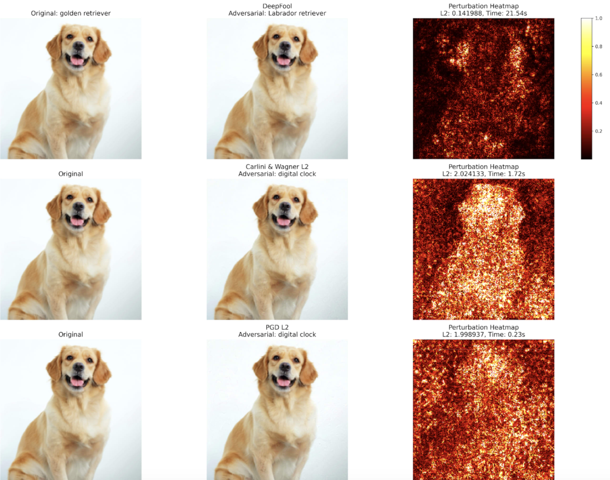
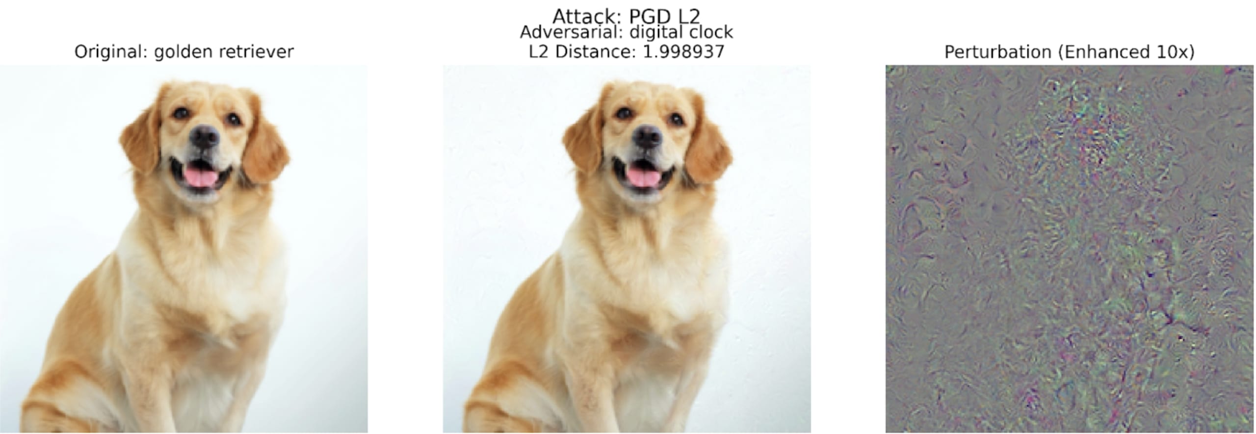
One natural goal of confusing the classifier is making the necessary perturbations without making the changes noticeable to the human eye. We estimate the magnitude of the perturbations using an L2 Distance – the distance of the image from the original, unmodified image, computed like so:
As a rule of thumb, for images with pixel RGB values each normalized to [0, 1] from [0,255], an L2 distance of < 5.0 would be our target, and > 10.0 would likely be human-noticeable. Using this non-normalized L2 distance means that, for larger images, you can generally expect a larger distance to be computed; however, this heuristic is acceptable for our little experiment.
Three Different Algorithms for Adversarial AI
Carlini & Wagner (C&W) L2 Attack: The Optimization Approach
The C&W attack, introduced in 2016, approaches adversarial example generation as an optimization problem. Instead of directly manipulating the image, it works in a transformed space that guarantees valid pixel values:
The attack minimizes a carefully crafted objective function that balances two goals:
Making minimal changes to the image (measured by L2 distance)
Forcing the model to output the target class

This is the core of the C&W attack's loss function:
This adversarial loss works like so:
In the targeted case, It tries to make the target class logit (
real) higher than the highest of all other logits (other).The
confidenceparameter controls how strongly the attack enforces misclassification. Higher values of confidence create adversarial examples that are classified with higher confidence but require larger perturbations.The
clamp(_, min=0)ensures the loss is only positive when misclassification hasn't been achieved with the desired confidence.The parameter c controls the trade-off between perturbation size and misclassification strength. The original C&W attack uses binary search to find the optimal value of c, starting with a small value and gradually increasing it until a successful adversarial example is found. This ensures that the adversarial example has the minimal perturbation necessary to fool the model.
PGDL2: The Iterative Approach
Projected Gradient Descent (PGD) with L2 constraints takes a different approach. Instead of complex optimization, it repeatedly:
Takes steps in the direction that increases the model's loss (hence the word ‘iterative’)
Projects the perturbation back onto an L2 ball to maintain a constraint on its size
An L2 ball is a geometric concept, representing all points that are within a certain Euclidean distance (the radius eps) from the center point. In the context of adversarial attacks, this center point is the original image, and the L2 ball represents all images that are within a specified L2 distance from the original. The constraint ensures that the adversarial perturbation is imperceptible to humans by keeping the L2 norm (Euclidean distance) of the perturbation below a threshold eps.
When we run our own sample image through this process:
The key insight of PGDL2 is its gradient normalization and projection steps:
The gradient normalization step normalizes the gradient to have a unit L2 norm (length of 1), preserving only its direction while discarding its magnitude; thus, we can control exactly how far we move in that direction using the alpha parameter. The gradient points in the direction of increasing loss, which for targeted attacks means decreasing the loss (hence the negative sign in cost = -loss(outputs, target_labels)).
After taking a step in the direction of the normalized gradient, the resulting image might exceed the L2 constraint (i.e., be outside the L2 ball). The projection step ensures that the perturbation remains within the allowed L2 ball. The projection is finding the closest point on or within the L2 ball to the current adversarial example.
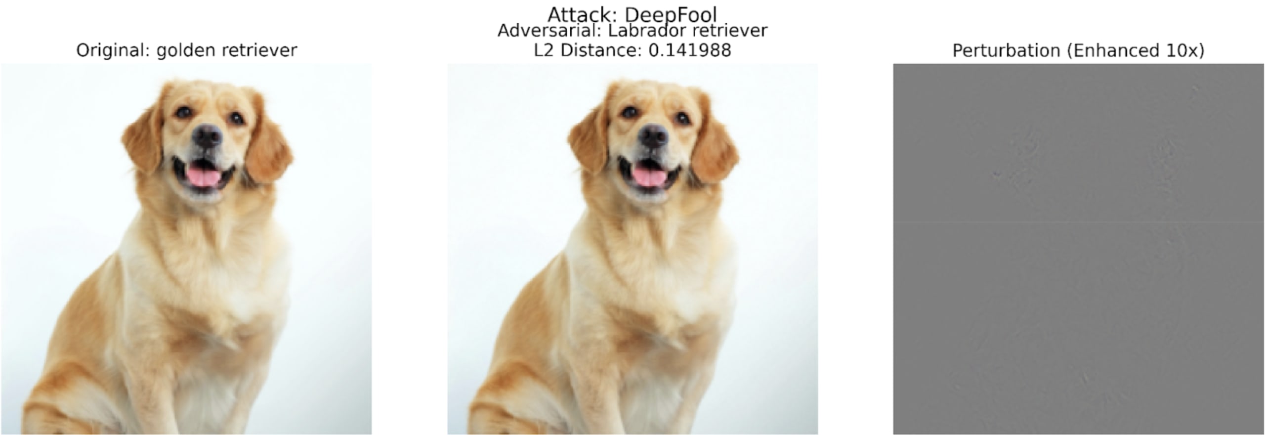
DeepFool: A Geometric Approach
DeepFool is not a neural network itself; it is a post-training attack method, meaning it doesn't require any training of its own. It can be used on already trained neural networks of any common architecture, including CNNs, ResNets, and transformers. The attack only requires that the model is differentiable so that the gradients can be computed.
In short, DeepFool takes a geometric perspective, iteratively finding the nearest decision boundary and stepping over it. It's an untargeted attack, meaning it simply tries to cause any misclassification rather than aiming for a specific target class.
Geometry in High Dimensions
Neural networks create complex decision boundaries in high-dimensional space. DeepFool approximates these boundaries locally as hyperplanes and then finds the shortest path to cross the nearest boundary, which represents the minimal perturbation needed to change the classification.
For a binary classifier, the decision boundary is a single hyperplane, and finding the minimal perturbation is straightforward: it's the projection of the input onto the hyperplane. For multi-class classifiers (such as our own ImageNet classifier in this example), DeepFool iteratively approximates the nearest decision boundary by linearizing the classifier at each step. Neural networks are highly nonlinear functions. However, locally (in a small neighborhood), they can be approximated by a linear function using the first-order Taylor expansion.
The attack iteratively applies small perturbations until the model's decision changes, ensuring the resulting adversarial example is close to the original image while successfully causing misclassification.
Comparing the Approaches
Let's look at how these attacks perform in practice:
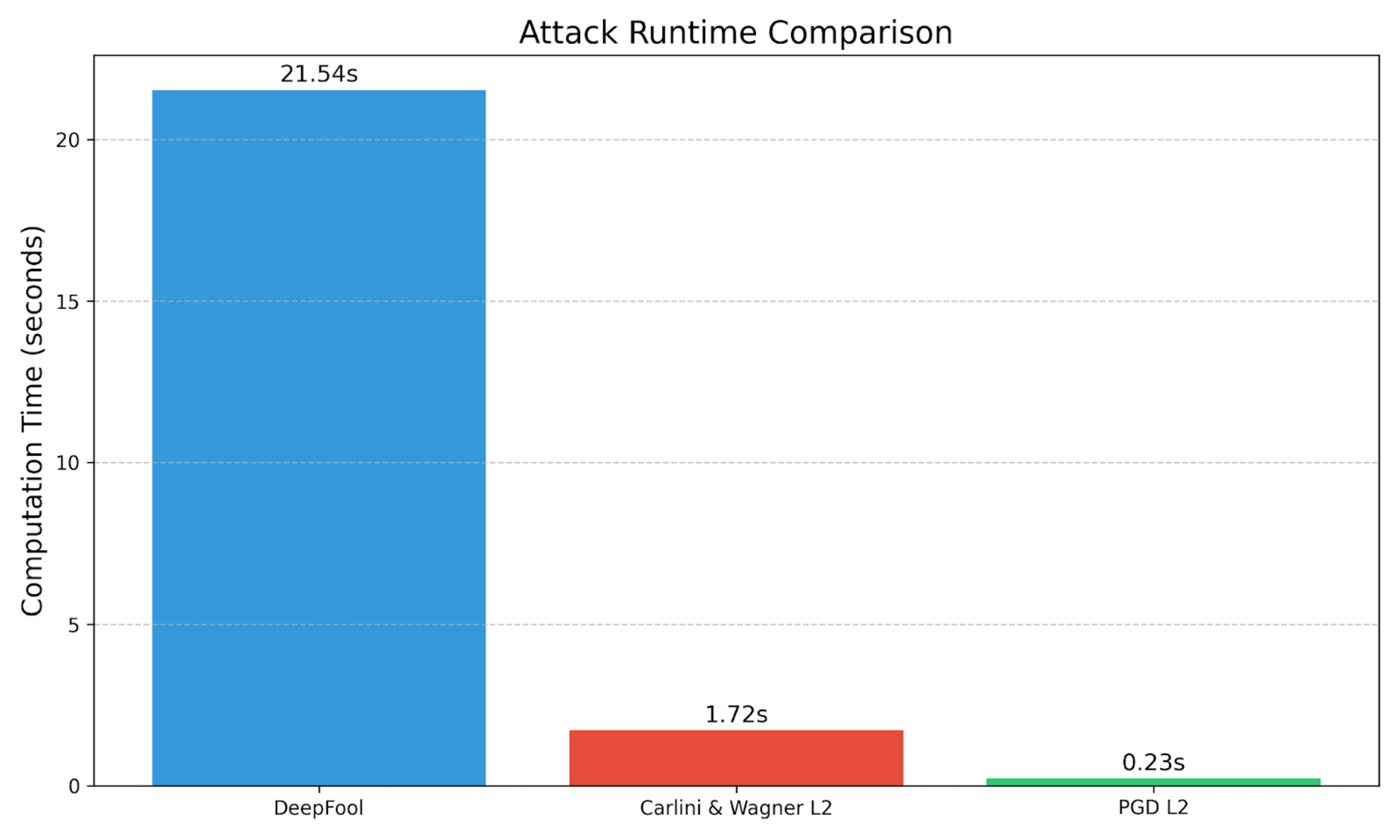
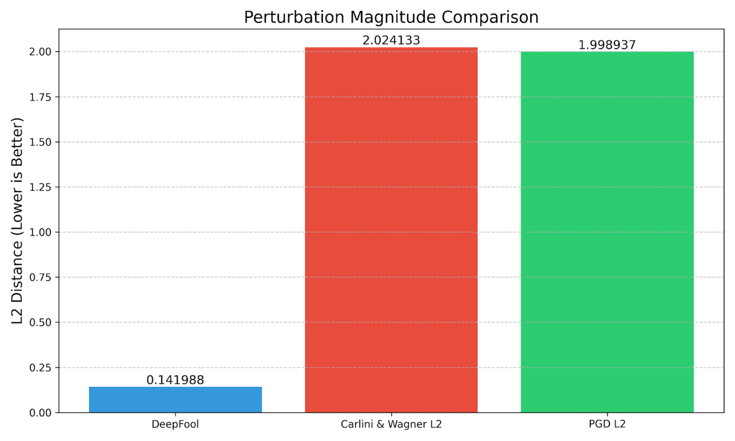
In our example case:
C&W offers a good balance of speed and perturbation size; it takes longer than PGDL2 to compute but has comparable L2 distance.
PGD has a lower L2 distance when targeting the digital clock class, and it runs faster than the C&W attack. PGD also produces a much higher confidence in its misclassification.
DeepFool takes the longest time to execute. It has the smallest L2 Distance, meaning the perturbation should be the least noticeable to the human eye. But, this is not an apples-to-apples comparison – DeepFool is an untargeted attack, and it is specifically searching for the nearest decision boundary. It fools the model such that it misclassifies the golden retriever as a labrador retriever, and these are two fairly similar classes.
Securing Against Adversarial Attacks
Adversarial attacks on image classifiers may not just be academic toys—they may be wake-up calls for the AI & ML security community. As we've seen, even slight perturbations can completely fool sophisticated models.
By understanding these attacks and using tools like Snyk to secure our ML pipelines, we can build more robust and trustworthy AI systems. Independent, open-source projects can apply for free access to enterprise-level tools with Snyk as a part of our Secure Developer Open Source program.
The code used in this article is available on GitHub: snyk-adversarial-inputs-to-image-classifiers
These attacks reveal a fundamental challenge in deep learning: our most powerful models can be fooled by carefully crafted perturbations that are imperceptible to humans. As we deploy AI systems in critical applications, we must:
Understand these vulnerabilities
Implement robust testing procedures
Deploy defense mechanisms
Regularly audit our systems
Understanding adversarial attacks highlights the security challenges facing AI systems. Beyond model-specific defenses, ensuring the security and integrity of the underlying code that builds, trains, and deploys these models is fundamental. Learn best practices for managing and securing AI-related code in Snyk's whitepaper: Taming AI Code: Securing Gen AI Development with Snyk